This is Part 1 of a two-part series.

This document covers setup, connectivity, and building an analytics read model — a single Flight SQL query materialised daily into a Delta table and served to BI.

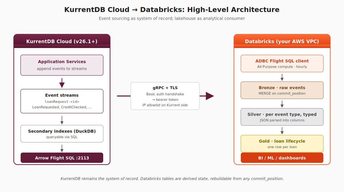
Part 2 extends the pattern into a full medallion pipeline (Bronze → Silver → Gold) with hourly incremental ingestion, per-event-type typed tables, and orchestrated Databricks Workflows for higher throughput and sub-daily refresh.

Background

Why Databricks for analytics

Databricks markets itself as a unified data and AI platform built on the lakehouse architecture — combining the openness and flexibility of data lakes with the performance and governance of data warehouses. Concretely, the platform brings together:

• Apache Spark for distributed compute at any scale
• Delta Lake for ACID transactions, time travel, and schema enforcement on cloud object storage
• Unity Catalog for unified governance over data, ML models, and AI assets
• Workflows for orchestrating scheduled and event-driven pipelines
• Collaborative notebooks in Python, SQL, R, and Scala
• Native BI integrations (PowerBI, Tableau, Looker) plus MLflow, vector search, and serving for ML and GenAI

For teams that need to derive analytical, BI, and ML value from large volumes of operational data, Databricks gives a single platform that scales horizontally, integrates broadly with the data ecosystem, and supports a wide range of workloads from interactive notebooks to scheduled production pipelines.

Why keep your events in KurrentDB

Events are first-class artifacts of modern systems — not derivative data. They are the canonical record of what happened, when, in what order, and what caused what. Three increasingly common patterns generate large volumes of these events:

• Event-sourced applications store state as an append-only sequence of events rather than mutating rows. Every domain change becomes an event; current state is derived by replay.
• Event-based business workflows — loan origination, order fulfilment, claims processing, employee onboarding, payment flows — emit events at every step. Orchestrated and choreographed processes that span services, teams, and time spans depend on these events for coordination, audit, and recovery.
• Agentic AI systems treat the event log as the agent’s durable memory and the substrate for evaluation. Reasoning traces, tool calls, intermediate decisions, and outcomes are recorded as events so the agent’s behaviour can be replayed, audited, fine-tuned, and held to a behavioural contract.

For all three patterns, KurrentDB is the durable, append-only, queryable home for that history. It offers properties no analytical store provides:

• Causal and temporal integrity — every event is timestamped and globally ordered. The exact sequence in which the business made decisions, or the agent took actions, is preserved.
• Replay from any point in time — derived state can be reconstructed deterministically from the event log. The lakehouse, dashboards, ML features, and AI agent context windows are all derived state.
• Real-time subscriptions for operational consumers — projections, alerts, downstream workflow steps, and agent runtimes consume the same events the analytical pipeline reads.
• Schema-on-read flexibility — events carry their structure as JSON, supporting upstream evolution without breaking historical replay.

Moving events directly into a relational warehouse loses this richness. The events become rows; the temporal causal chain becomes inferred. KurrentDB preserves it, and feeds the lakehouse on demand.

The pattern this whitepaper describes

This document describes the pattern most operationally-mature teams adopt:

• KurrentDB remains the system of record for events. Operational systems write to it; real-time projections read from it.
• Databricks becomes a downstream analytical consumer. Events are pulled into Databricks via Arrow Flight SQL on a schedule (hourly or faster), organised using the medallion (bronze / silver / gold) architecture, and served to BI, ML, and ad-hoc analytics.
• Because every byte landed in Databricks is recoverable from KurrentDB, the lakehouse is treated as derived state — rebuildable from any historical point on demand.

The pattern preserves the strengths of both platforms: KurrentDB’s durability, causality, and replay; Databricks’ scale, BI integration, and analytical compute.

Architecture overview

At the highest level, the pattern has three pieces: an event-producing source (KurrentDB), a transport (Arrow Flight SQL over gRPC + TLS), and an analytical consumer (Databricks).

Example Loan Application system analytical read models built from events in a Kurrent Cloud hosted database

Source — KurrentDB. Application services append events to streams (e.g., loanRequest-<id>). KurrentDB indexes these events into a queryable form via embedded secondary indexes (DuckDB-backed in v25.1+) and exposes them through the Arrow Flight SQL endpoint.

Transport — Arrow Flight SQL. A gRPC + TLS protocol designed to stream large columnar result sets efficiently. Authentication is via basic-auth, which returns a bearer token used for the rest of the session. Connections originate from Databricks compute and terminate at the KurrentDB cluster on port 2113.

Consumer — Databricks. A scheduled job runs in your Databricks workspace, pulls events via the Arrow Flight SQL client (adbc-driver-flightsql), and lands them into a medallion structure: Bronze (raw events as ingested), Silver (per-event-type tables with JSON parsed into typed columns), and Gold (business-level analytical projections). BI tools, ML pipelines, and dashboards consume the Gold layer.
KurrentDB is the system of record. The Databricks tables are derived state — reproducible by replaying kdb.records from any historical position.

Glossary and definitions

kdb.records

KurrentDB Flight SQL virtual table exposing every event with stream, category, schema_name, data, metadata, created_at (Unix UTC ms), and log_position.

log_position

Monotonic 64-bit global position. The canonical event-ordering and ingestion anchor exposed by kdb.records

ADBC

Arrow Database Connectivity — a Python DB-API 2.0 compatible driver layer that constructs the Flight SQL protocol’s protobuf messages on your behalf. The whitepaper uses adbc-driver-flightsql.

Arrow Flight SQL

gRPC-based protocol for streaming columnar query results as Arrow record batches.

Customer-managed VPC

Databricks deployment model where infrastructure runs in your AWS account, not Databricks’.

NAT Gateway

AWS service providing outbound internet for private subnets via Source NAT to an Elastic IP.

All-Purpose compute

Classic Databricks compute (vs. serverless); runs in your VPC; full network control.

Secondary indexes

KurrentDB feature (v25.1+) that builds DuckDB-backed indexes over category and event type.

Medallion

Bronze (raw) → Silver (cleaned, typed) → Gold (aggregated) data layering convention.

HWM

High-Water Mark. The last successfully-processed offset, persisted between job runs.

Read model

A single materialised view tailored to a specific analytical question, typically rebuilt on a schedule.

Prerequisites

• A KurrentDB v26.1 or later environment accessible to Databricks. v26.1 introduced Arrow Flight SQL protocol support. The examples in this whitepaper use KurrentDB Cloud, but any reachable v26.1+ cluster (self-hosted, on-premises, or in a different cloud) works the same way.
• A KurrentDB user with admin privileges, required to query the $all-equivalent virtual tables via secondary indexes.
• A Databricks workspace with the ability to call out to external services for data ingestion. Examples use Databricks on AWS with a customer-managed VPC, but the pattern works identically on Azure Databricks and Databricks on GCP as long as the workspace can reach the KurrentDB endpoint.
• Network reachability from the Databricks compute environment to the KurrentDB Flight SQL endpoint on port 2113, including any IP allowlists on the Kurrent side.

Creating a Databricks Environment (optional)

Skip this section if you already have a Databricks workspace with All-Purpose compute capability and outbound internet egress.

This section walks through provisioning a fresh Databricks workspace on AWS suitable for this pattern. The same general approach applies on Azure and GCP, following Databricks documentation for the corresponding deployment models.

Choose the right deployment model

Not all Databricks subscription paths support the pattern in this whitepaper. To run a Python notebook with adbc-driver-flightsql against an external gRPC endpoint, you need classic (All-Purpose) compute with controllable network egress. Two common starting points do not provide this:

• Databricks Free Edition — serverless-only, restricted egress, non-commercial use.
• AWS Marketplace Pay-as-you-go (SaaS) — Databricks-hosted infrastructure, serverless-only, no all-purpose compute.

The required path is Premium tier deployed into your own AWS account via AWS Marketplace (or directly via Databricks’s “Continue with your cloud account” sign-up flow). The deployment runs CloudFormation in your AWS account, which creates a VPC with subnets, IGW, NAT Gateway, IAM roles, and the workspace itself.

Sign up

1. Go to https://www.databricks.com/try-databricks or AWS Marketplace.
2. On the cloud-provider step, choose AWS and select the “Deploy in my own cloud account” flow (the wording evolves; look for any option that mentions CloudFormation or your AWS account).
3. Sign in to AWS, accept and launch the CloudFormation template.
4. Choose a region — co-locate with your KurrentDB cluster’s region to minimise latency.
5. Wait ~10–15 minutes for the stack to complete.

After the workspace is provisioned, verify in the Databricks UI: Compute → All-purpose tab should exist. In the AWS console, VPC → Your VPCs should show a new VPC with a custom CIDR (e.g. 10.0.0.0/16).

Verify the VPC has working egress

The CloudFormation template usually creates a NAT Gateway, but some templates omit it to reduce trial costs. Verify in AWS Console:

• VPC → Internet Gateways — one should be Attached to your Databricks VPC.
• VPC → NAT Gateways — at least one should exist in the Databricks VPC, in state Available, with an Elastic IP attached.
• VPC → Route Tables — the private subnet route table should have 0.0.0.0/0 → nat-XXXX.

If the NAT Gateway is missing, create one: NAT Gateways → Create NAT gateway, choose a public subnet, allocate an Elastic IP, Create. Then update private route tables to point 0.0.0.0/0 at the new NAT.

Create an All-Purpose compute cluster

In the Databricks workspace:

1. Compute → All-purpose → Create compute
2. Settings:
   • Compute name: kurrent-ingest (or anything descriptive)
   • Policy: Personal Compute
   • Uncheck Machine Learning (not needed; saves startup time)
   • Databricks Runtime: 15.4 LTS or 16.x LTS
   • Node type: i3.xlarge (or smallest available)
   • Terminate after: 30 minutes of inactivity (NOTE: you may wish to adjust this timeout period to reflect your own preferences and organizational practices)
   • Advanced → Access mode: Dedicated (Single user) — yourself
3. Create compute. Wait ~3–5 minutes for the cluster to reach Running.

Configuring your KurrentDB Cloud Cluster (optional)

Skip this section if you already have a KurrentDB cluster reachable from your Databricks workspace.

Provision the cluster

Follow the official Kurrent Cloud documentation to provision a v26.1+ cluster in the region closest to your Databricks workspace. The Cloud UI walks through cluster sizing, region, network configuration, and version selection.

Allowlist the Databricks public IP

KurrentDB Cloud enforces IP-based access control. Outbound traffic from Databricks reaches Kurrent’s edge with the source IP of your VPC’s NAT Gateway Elastic IP — that’s what needs to be in the allowlist.

Find your Databricks public IP — two ways. Use either method; the live test is the source of truth, especially if your VPC has multiple NAT Gateways.

Method A — AWS Console. VPC → NAT Gateways → filter by your Databricks VPC. Copy each Elastic IP Address. If multiple NATs exist (typical HA setup), collect them all.
Method B — From a Databricks notebook attached to your cluster. In a fresh cell:

import urllib.request
ip = urllib.request.urlopen('https://checkip.amazonaws.com', timeout=10).read().decode().strip()
print(f"Outbound public IP: {ip}")

This is the IP every external service will see for the current cluster session.
Add to Kurrent Cloud. In the Kurrent Cloud console:

1. Open your cluster
2. Navigate to the Network (or Security / Access Control) tab
3. Add each NAT Gateway EIP as a /32 CIDR (e.g., 52.10.20.30/32)
4. Save, and confirm the entry appears in the saved state
5. Allow ~10 minutes for propagation

NOTE: Don’t forget other firewall layers. If your enterprise has an additional egress firewall (corporate proxy, WAF, AWS Network Firewall, etc.) between your Databricks VPC and the public internet, the Databricks public IP needs to be allowed there too. Coordinate with whoever owns those layers before testing.
NAT Gateway Elastic IPs are stable for the life of the NAT Gateway. Document them so the Kurrent allowlist doesn’t silently break if VPC infrastructure is later rebuilt.

Testing the Connection from Databricks

Before building application code, verify the end-to-end network path is healthy: Databricks compute → NAT Gateway → public internet → Kurrent Cloud allowlist → KurrentDB cluster → authentication → event read. This catches infrastructure issues in isolation, before they’re entangled with ingestion logic.

The test uses the native KurrentDB Python client (kurrentdbclient), which is simpler for connectivity smoke-testing and exercises the same gRPC + TLS + basic-auth handshake path that Flight SQL uses.

Run the connection-testing notebook

Open a new notebook attached to your All-Purpose compute cluster and run the following three cells.

Cell 1 — install client and refresh the kernel.

%pip install --upgrade "protobuf>=6.31.0"
%pip install kurrentdbclient
dbutils.library.restartPython()

NOTE: The explicit protobuf upgrade is required because Databricks Runtime ships protobuf 5.x for PySpark compatibility, but kurrentdbclient is compiled against protobuf 6.x. Without the upgrade you get VersionError: Detected mismatched Protobuf Gencode/Runtime major versions. The restartPython() ensures the new protobuf actually loads into the kernel.

Cell 2 — confirm the outbound IP (should match what you allowlisted in the previous section):

import urllib.request
ip = urllib.request.urlopen('https://checkip.amazonaws.com', timeout=10).read().decode().strip()
print(f"Outbound public IP: {ip}")

Cell 3 — the layered connectivity diagnostic. Replace CLUSTER_HOST, USERNAME, PASSWORD with values for your cluster.

"""
KurrentDB connectivity test from Databricks.
Layered diagnostic: each step prints ✓ or ✗ so you can pinpoint failures.
"""
import socket
from kurrentdbclient import KurrentDBClient

CLUSTER_HOST = "<cluster-id>.mesdb.eventstore.cloud"
CLUSTER_PORT = 2113
USERNAME = "admin"
PASSWORD = "changeit"

# Layer 1 — DNS resolution
print(f"[1/4] DNS resolution for {CLUSTER_HOST} ...")
try:
    ip = socket.gethostbyname(CLUSTER_HOST)
    print(f"      ✓ Resolved to {ip}")
except socket.gaierror as e:
    print(f"      ✗ DNS failed: {e}")

# Layer 2 — Raw TCP (proves NAT egress + Kurrent allowlist)
print(f"[2/4] TCP connection to {CLUSTER_HOST}:{CLUSTER_PORT} ...")
try:
    with socket.create_connection((CLUSTER_HOST, CLUSTER_PORT), timeout=10):
        print(f"      ✓ TCP handshake completed")
except OSError as e:
    print(f"      ✗ TCP failed: {e}")

# Layer 3 — gRPC + TLS + auth
uri = f"kurrentdb+discover://{USERNAME}:{PASSWORD}@{CLUSTER_HOST}:{CLUSTER_PORT}"
print(f"[3/4] gRPC connect (TLS + cluster discovery + auth) ...")
client = None
try:
    client = KurrentDBClient(uri=uri)
    print(f"      ✓ Client constructed and connected")
except Exception as e:
    print(f"      ✗ Failed: {type(e).__name__}: {e}")

# Layer 4 — Read from $all (proves auth + read permission + data path)
print(f"[4/4] Reading first 5 events from $all ...")
if client is None:
    print(f"      ⊘ Skipped (no client from layer 3)")
else:
    try:
        events = []
        for ev in client.read_all():
            events.append(ev)
            if len(events) >= 5:
                break
        if not events:
            print(f"      ✓ Connected, but $all is empty (no events written yet)")
        else:
            print(f"      ✓ Read {len(events)} event(s):")
            for i, ev in enumerate(events, 1):
                stream = getattr(ev, "stream_name", "?")
                etype  = getattr(ev, "type", "?")
                cpos   = getattr(ev, "log_position", "?")
                print(f"        [{i}]  stream={stream}  type={etype}  log_position={cpos}")
    except Exception as e:
        print(f"      ✗ Read failed: {type(e).__name__}: {e}")
    finally:
        client.close()

print()
print("=" * 60)
print("Connectivity test complete — review ✓/✗ above")
print("=" * 60)

What success looks like

All four layers should print ✓ and the final block should show five sample events. For our demo cluster the output will look similar to:

[1/4] DNS resolution for d87...mesdb.eventstore.cloud ...
✓ Resolved to 15.157.248.16
[2/4] TCP connection ...
✓ TCP handshake completed
[3/4] gRPC connect ...
✓ Client constructed and connected
[4/4] Reading first 5 events from $all ...
✓ Read 5 event(s):
[1]  stream=loanRequest-b5959eea-...  type=LoanRequested  log_position=9401
[2]  stream=loanRequest-9bffd3d3-...  type=LoanRequested  log_position=10270
...

Diagnosing failures

1 — DNS

Wrong hostname; or VPC DNS resolution misconfigured

2 — TCP timeout

NAT Gateway missing or misrouted; or Kurrent allowlist excluding your NAT EIP

2 — TCP refused

Port 2113 not exposed; cluster down

3 — TLS / auth error

Cert verification failed; wrong username/password

4 — Permission error

User not admin (required for $all reads in v26.x)

Configuring the Databricks Workspace

With connectivity verified, provision the Unity Catalog resources your ingestion will use. This section uses the simplest viable setup — hardcoded credentials in notebooks for clarity. In production, move credentials into Databricks secret scopes and use a service principal for scheduled jobs; that hardening is straightforward to layer on once the pipeline is working end-to-end.

Create the catalog (via UI)

Catalog creation depends on whether your account uses Default Storage (Databricks manages backing storage automatically) or a customer-configured metastore root (you provide an S3 bucket). The UI handles both transparently; SQL CREATE CATALOG without a MANAGED LOCATION clause only works on accounts with a metastore root URL configured. Use the UI to avoid that branch and stay portable across account types.

1. Left nav → Catalog
2. Click Create Catalog (top right of Catalog Explorer)
3. Name: loan_lakehouse
4. Type: Standard
5. Storage location: leave blank to use Default Storage, or pick a pre-configured External Location if your account uses one
6. Click Create

Create the schemas (via SQL)

Schemas inherit the catalog’s storage configuration, so SQL creation works on any account type. Open the workspace’s SQL Editor (or a notebook attached to your cluster) and run:

USE CATALOG loan_lakehouse;

CREATE SCHEMA IF NOT EXISTS bronze;
CREATE SCHEMA IF NOT EXISTS silver;
CREATE SCHEMA IF NOT EXISTS gold;
CREATE SCHEMA IF NOT EXISTS ops;

CREATE VOLUME IF NOT EXISTS ops._checkpoints;

The four schemas correspond to the medallion layers plus an ops schema for operational state (high-water marks, dead-letter tables). The _checkpoints managed Volume under ops is where the Silver streaming checkpoints land — Unity Catalog /Volumes/… paths resolve to Volume objects, not arbitrary folders, so the Volume has to exist before the streams write to it.

Verify your user can write to the catalog

Run a quick test:

CREATE TABLE loan_lakehouse.ops._smoke_test (note STRING) USING DELTA;
INSERT INTO loan_lakehouse.ops._smoke_test VALUES ('hello');
SELECT * FROM loan_lakehouse.ops._smoke_test;
DROP TABLE loan_lakehouse.ops._smoke_test;

If all four statements succeed, you have the permissions you need. If any fails, you’ll need additional Unity Catalog privileges granted by a metastore admin.

NOTE: That’s the entire workspace provisioning step for this example. Production environments add service principals, secret scopes, and access-controlled grants — see the Databricks security documentation for those patterns.

Creating an Analytics Read Model

The simplest possible analytics pattern: execute a SQL query directly against KurrentDB’s Flight SQL endpoint on a daily schedule, materialise the result to a Databricks Delta table, and serve that to BI. This is sometimes called the “read model” pattern because you’re building a single materialised view tailored to a specific analytical question.

This pattern works well when:

• The analytical question is well-defined and stable
• The full result set is small enough to compute in one pass (KurrentDB’s query engine returns a single Arrow result)
• You don’t need cross-source joins with other Databricks data

For our event-sourced loan-origination example, a typical read model is one row per loan with its full lifecycle state — useful for ops dashboards, batch reporting, and downstream BI.

The Loan Status SQL

The query below runs against KurrentDB’s Flight SQL endpoint. It pulls every event in the loanRequest category, splits them by their schema name (event type) into the five lifecycle stages, full-outer-joins them on stream identifier, and adds a derived age_binned column. The result is one row per loan with all known state from across its lifecycle.

SELECT *,
       CASE
           WHEN age < 15 THEN '0 - 14 Years'
           WHEN age < 25 THEN '15 - 24 Years'
           WHEN age < 35 THEN '25 - 34 Years'
           WHEN age < 45 THEN '35 - 44 Years'
           WHEN age < 55 THEN '45 - 54 Years'
           WHEN age < 65 THEN '55 - 64 Years'
           WHEN age < 75 THEN '65 - 74 Years'
           WHEN age < 85 THEN '75 - 84 Years'
           WHEN age < 95 THEN '85 - 94 Years'
           ELSE '95+ Years'
       END AS age_binned
FROM (
    SELECT loanrequestid,
           amount::int amount,
           nationalid,
           "name",
           gender,
           age::int age,
           maritalstatus,
           dependents::int dependents,
           levelofeducation,
           employername,
           jobtitle,
           jobseniority::float jobseniority,
           income::int income,
           address_street,
           address_city,
           address_region,
           address_country,
           address_postalcode,
           CAST(loanrequestedtimestamp AS TIMESTAMP) loanrequestedtimestamp,
           loanproductid::int loanproductid,
           score::int score,
           CAST(creditcheckedtimestamp AS TIMESTAMP) creditcheckedtimestamp,
           CAST(loanautomateddecisiontimestamp AS TIMESTAMP) loanautomateddecisiontimestamp,
           CAST(loanmanualdecisiontimestamp AS TIMESTAMP) loanmanualdecisiontimestamp,
           approvername,
           creditscoresummary::string creditscoresummary,
           incomeandemploymentsummary::string incomeandemploymentsummary,
           loantoincomesummary::string loantoincomesummary,
           maritalstatusanddependentssummary::string maritalstatusanddependentssummary,
           recommendedfurtherinvestigation::string recommendedfurtherinvestigation,
           summarizedby::string summarizedby,
           CAST(summarizedat AS TIMESTAMP) summarizedat,
           COALESCE(manual.laststatus, summary.laststatus, auto.laststatus,
                    cc.laststatus, lr.laststatus, 'UNKNOWN') laststatus
    FROM (
        SELECT stream,
               data::json->>'LoanRequestID' loanrequestid,
               data::json->>'Amount' amount,
               data::json->>'Name' "name",
               data::json->>'NationalID' nationalid,
               data::json->>'Gender' gender,
               data::json->>'Age' age,
               data::json->>'MaritalStatus' maritalstatus,
               data::json->>'Dependents' dependents,
               data::json->>'LevelOfEducation' levelofeducation,
               data::json->>'EmployerName' employername,
               data::json->>'JobTitle' jobtitle,
               data::json->>'JobSeniority' jobseniority,
               data::json->>'Income' income,
               data::json->'Address'->>'Street' address_street,
               data::json->'Address'->>'City' address_city,
               data::json->'Address'->>'Region' address_region,
               data::json->'Address'->>'Country' address_country,
               data::json->'Address'->>'PostalCode' address_postalcode,
               data::json->>'LoanRequestedTimestamp' loanrequestedtimestamp,
               data::json->>'LoanProductID' loanproductid,
               schema_name laststatus
        FROM kdb.records
        WHERE category = 'loanRequest'
          AND schema_name = 'LoanRequested'
    ) AS lr
    FULL OUTER JOIN (
        SELECT stream,
               data::json->>'Score' score,
               data::json->>'CreditCheckedTimestamp' creditcheckedtimestamp,
               schema_name laststatus
        FROM kdb.records
        WHERE category = 'loanRequest'
          AND schema_name = 'CreditChecked'
    ) AS cc ON lr.stream = cc.stream
    FULL OUTER JOIN (
        SELECT stream,
               data::json->>'LoanAutomatedDecisionTimestamp' loanautomateddecisiontimestamp,
               schema_name laststatus
        FROM kdb.records
        WHERE category = 'loanRequest'
          AND schema_name IN ('LoanAutomaticallyApproved', 'LoanAutomaticallyDenied', 'LoanApprovalNeeded')
    ) AS auto ON cc.stream = auto.stream
    FULL OUTER JOIN (
        SELECT stream,
               data::json->>'ApproverName' approvername,
               data::json->>'LoanManualDecisionTimestamp' loanmanualdecisiontimestamp,
               schema_name laststatus
        FROM kdb.records
        WHERE category = 'loanRequest'
          AND schema_name IN ('LoanManuallyApproved', 'LoanManuallyDenied')
    ) AS manual ON auto.stream = manual.stream
    FULL OUTER JOIN (
        SELECT stream,
               data::json->>'CreditScoreSummary' creditscoresummary,
               data::json->>'IncomeAndEmploymentSummary' incomeandemploymentsummary,
               data::json->>'LoanToIncomeSummary' loantoincomesummary,
               data::json->>'MaritalStatusAndDependentsSummary' maritalstatusanddependentssummary,
               data::json->>'RecommendedFurtherInvestigation' recommendedfurtherinvestigation,
               data::json->>'SummarizedBy' summarizedby,
               data::json->>'SummarizedAt' summarizedat,
               schema_name laststatus
        FROM kdb.records
        WHERE category = 'loanRequest'
          AND schema_name = 'AutomatedSummary'
    ) AS summary ON manual.stream = summary.stream
) AS loanRequest;

NOTE: The explicit ::string casts on the AutomatedSummary fields matter: when no events of that type have been written yet (or when an entire result column comes back all-NULL), the column otherwise gets inferred as VOID, which Spark can’t materialise into a typed Delta column. Casting at the source keeps the Arrow result strongly-typed.

NOTE: This SQL is intended to run on the KurrentDB side, not in Databricks. The KurrentDB Flight SQL engine (DuckDB-backed) executes the joins and JSON projections natively. Databricks just receives the result as a single Arrow table.

Pre-create the Gold loan_status table

Even with the source-side ::string casts, columns the read model derives can come back without inferable types on a cold cluster (no AutomatedSummary events yet, for example). Pre-creating the Gold table with explicit types eliminates that class of failure entirely and gives BI tools a stable schema to bind to from day one.

In the SQL Editor on your kurrent-ingest cluster (or any notebook attached to it), run:

CREATE TABLE IF NOT EXISTS loan_lakehouse.gold.loan_status (
    loanrequestid                       STRING,
    amount                              INT,
    nationalid                          STRING,
    name                                STRING,
    gender                              STRING,
    age                                 INT,
    maritalstatus                       STRING,
    dependents                          INT,
    levelofeducation                    STRING,
    employername                        STRING,
    jobtitle                            STRING,
    jobseniority                        FLOAT,
    income                              INT,
    address_street                      STRING,
    address_city                        STRING,
    address_region                      STRING,
    address_country                     STRING,
    address_postalcode                  STRING,
    loanrequestedtimestamp              TIMESTAMP,
    loanproductid                       INT,
    score                               INT,
    creditcheckedtimestamp              TIMESTAMP,
    loanautomateddecisiontimestamp      TIMESTAMP,
    loanmanualdecisiontimestamp         TIMESTAMP,
    approvername                        STRING,
    creditscoresummary                  STRING,
    incomeandemploymentsummary          STRING,
    loantoincomesummary                 STRING,
    maritalstatusanddependentssummary   STRING,
    recommendedfurtherinvestigation     STRING,
    summarizedby                        STRING,
    summarizedat                        TIMESTAMP,
    laststatus                          STRING,
    age_binned                          STRING
) USING DELTA;

Column names match the aliases used by the SQL. Once this table exists, the read-model notebook below overwrites its contents on each daily run while preserving the schema.

Read-model notebook

Create a notebook named daily_loan_status_refresh.

Cell 1 — install the ADBC Flight SQL driver:

%pip install adbc-driver-flightsql
dbutils.library.restartPython()

The driver handles the Flight SQL protocol’s protobuf-wrapped command messages, basic-auth handshake, TLS, and Arrow result streaming. Raw pyarrow.flight cannot be used directly — Kurrent’s Flight SQL handler expects properly-serialized CommandStatementQuery messages, not raw SQL bytes.

Cell 2 — execute the SQL on KurrentDB, materialise to Gold:

"""
Daily loan-status read model.
Executes the loan-status SQL against KurrentDB's Flight SQL engine via ADBC,
materialises the result to the pre-created Delta table.
"""
import base64
import adbc_driver_flightsql.dbapi as dbapi
from adbc_driver_flightsql import DatabaseOptions

CLUSTER_HOST = "<cluster-id>.mesdb.eventstore.cloud"
CLUSTER_PORT = 2113
USERNAME = "admin"
PASSWORD = "changeit"

LOAN_STATUS_SQL = """
<paste the full SQL from the previous section here>
"""

# Authenticate via a Basic auth header. The adbc-driver-flightsql driver does
# not negotiate basic auth on its own; the standard pattern is to encode the
# credentials and pass them as the Authorization header on every call.
auth_str = f"{USERNAME}:{PASSWORD}"
encoded_auth = base64.b64encode(auth_str.encode()).decode()

conn = dbapi.connect(
f"grpc+tls://{CLUSTER_HOST}:{CLUSTER_PORT}",
db_kwargs={
DatabaseOptions.AUTHORIZATION_HEADER.value: f"Basic {encoded_auth}",
},
)

cur = conn.cursor()
cur.execute(LOAN_STATUS_SQL)
arrow_table = cur.fetch_arrow_table()

print(f"Fetched {arrow_table.num_rows} loan records from KurrentDB")

# Overwrite the pre-created Gold table. Schema is preserved because the table
# already exists; we are not passing overwriteSchema.
df = spark.createDataFrame(arrow_table.to_pandas())
(df.write
.format("delta")
.mode("overwrite")
.saveAsTable("loan_lakehouse.gold.loan_status"))

print(f"Wrote {df.count()} rows to loan_lakehouse.gold.loan_status")

The ADBC dbapi interface is a standard DB-API 2.0 cursor pattern (familiar to anyone who’s used psycopg2 or sqlite3), but cur.fetch_arrow_table() returns a pyarrow.Table directly — no intermediate Python row materialisation, which keeps memory bounded even for large result sets.

Investigate the loaded data

Once the notebook has run, the loan_status table is queryable from any notebook, the SQL Editor, or any connected BI tool. A few starter queries to sanity-check the load and exercise the shape of the data:

-- Row count
SELECT COUNT(*) FROM loan_lakehouse.gold.loan_status;

-- Spot-check: applicant name, city, and where they are in the lifecycle
SELECT name, address_city, laststatus
FROM loan_lakehouse.gold.loan_status;

-- Average requested loan amount by age band
SELECT
age_binned,
AVG(amount) AS average_loan_amount
FROM loan_lakehouse.gold.loan_status
GROUP BY age_binned
ORDER BY age_binned;

The third query is a useful first BI chart: requested-amount-by-age is a single bar chart that confirms both that the read model loaded correctly and that the age_binned derivation is working.

Schedule the notebook daily

1. Workflows → Create Job
2. Name: daily_loan_status_refresh
3. Task: notebook task pointing at daily_loan_status_refresh, on your kurrent-ingest cluster
4. Schedule: scheduled, Quartz cron 0 0 6 * * ? (every day at 06:00 UTC, or whichever time aligns with your operational schedule)
5. Run as: your user (in production, a service principal)
6. Save

The job will run nightly; the loan_lakehouse.gold.loan_status table will be fully refreshed each run. Connect PowerBI, Tableau, or your dashboarding tool of choice to that table.

This is the entire read model. No medallion layers, no incremental processing, no MERGE logic. Two files: a notebook and a job. The trade-off is full re-compute on every run, which is fine for daily refresh of a moderately-sized result; for larger volumes or sub-daily refresh, the medallion pipeline in the next section is the right pattern.

Conclusion

This document walked through the end-to-end path from a KurrentDB cluster to a queryable Databricks Delta table: provisioning the infrastructure, verifying connectivity, configuring Unity Catalog, and building an analytics read model that materialises a single Flight SQL query into a Gold table on a daily schedule. The read-model pattern is deliberately simple — two files, no medallion layers, no incremental bookkeeping — and is the right starting point when the analytical question is stable and the event volume fits a full-refresh cadence.

In Part 2, we extend this foundation into a proper medallion analytics pipeline for teams that need hourly (or faster) refresh, incremental ingestion with high-water-mark tracking, per-event-type Silver tables with typed columns, and a Gold lifecycle table built from parallel Silver projections — all orchestrated as a single Databricks Workflow with deterministic replay from KurrentDB.